Social network analysis has become rather popular over the last five (or so) years; the proliferation of different manifestations of the social web has propelled it from being a relatively esoteric method in the social sciences to become something that has touched many people, if only superficially. The network visualisation – not necessarily a social network, e.g. Chris Harrison’s internet map – has become a symbol of the transformation in connectivity and modes of interaction that modern hardware, software and infrastructure has brought.
This is all very well, but I want more than network visualisations and computed statistics such as network density or betweenness centrality. The alluring visualisation that is the sociogram tends to leave me rather non-plussed.
Now, don’t get me wrong: I’m not against this stuff and I’m not attacking the impressive work of people like Martin Hawksey or Tony Hirst, the usefulness of tools like SNAPP or recent work on the Open University (UK) SocialLearn data using the NAT tool. I just want more and I want an approach which opens up the possibility of model building and testing, of hypothesis testing, etc. I want to be able to do this to make more sense of the data.
Warning:
this article assumes familiarity with Social Network Analysis.
Tools and Method
Several months ago, I became rather excited to find that exactly this kind of approach – social network modelling – has been a productive area of social science research and algorithm development for several years and that there is now a quite mature package called “ergm” for R. This package allows its user to propose a model for small-scale social processes and to evaluate the degree of fit to an observed social network. The mathematical formulation involves an exponential to calculate probability hence the approach is known as “Exponential Random Graph Models” (ERGM). The word “random” captures the idea that the actual social network is only one of many possibilities that could emerge from the same social forces, processes, etc and that this randomness is captured in the method.
I have added some what I have found to be the most useful papers and a related book to a Mendeley group; please consult these for an outline of the historical development of the ERGM method and for articles introducing the R package.
The essential idea is quite simple, although the algorithms required to turn it into a reality are quite scary (and I don’t pretend to understand enough to do proper research using the method). The idea is to think about some arguable and real-world social phenomena at a small scale and to compute what weightings apply to each of these on the basis of a match between simulations of the overall networks that could emerge from these small-scale phenomena and a given observed network. Each of the small-scale phenomena must be expressed in a way that a statistic can be evaluated for it and this means it must be formulated as a sub-graph that can be counted.
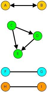
The diagram above illustrates three kinds of sub-graph that match three different kinds of evolutionary force on an emerging network. Imagine the arrows indicate something like “I consider them my friend”, although we can use the same formalism for less personal kinds of tie such as “I rely on” or even the relation between people and resources.
- The idea of mutuality is captured by the reciprocal relationships between A and B. Real friendship networks should be high in mutuality whereas workplace social networks may be less mutual.
- The idea of transitivity is captured in the C-D-E triangle. This might be expressed as “my friend’s friend is my friend”.
- The idea of homophily is captured in the bottom pair of subgraphs, which show preference for ties to the same colour of person. Colour represents any kind of attribute, maybe a racial label for studies of community polarisation or maybe gender, degree subject, football team… This might be captured as “birds of a feather fly together”.
One of the interesting possibilities of social network modelling is that it may be able to discover the likely role of different social processes, which we cannot directly test, with qualitatively similar outcomes. For example, both homophily and transitivity favour the formation of cohesive groups. A full description of research using ERGMs to deal with this kind of question is “Birds of a Feather, or Friend of a Friend? Using Exponential Random Graph Models to Investigate Adolescent Social Networks” (Goodreau, Kitts & Morris): see the Mendeley group.
A First Experiment
In the spirit of active learning, I wanted to have a go. This meant using relatively easily-available data about a community that I knew fairly well. Twitter follower networks are fashionable and not too hard to get, although the API is a bit limiting, so I wrote some R to crawl follower/friends and create a suitable data structure for use with the ERGM package.
Several evenings later I concluded that a network defined as followers of the EC-TEL 2012 conference was unsuitable. The problem seems to be that the network is not at all homogeneous while at the same time there are essentially no useful person attributes to use; the location data is useless and the number of tweets is not a good indicator of anything. Without some quantitative or categorical attribute you are forced to use models that assume homogeneity. Hence nothing I tried was a sensible fit.
Lesson learned: knowledge of person (vertex) attributes is likely to be important.
My second attempt was to consider the Twitter network between CETIS staff and colleagues in the JISC Innovation Group. In this case, I know how to assign one attribute that might be significant: team membership.
Without looking at the data, it seems reasonable to hypothesise as follows:
- We might expect a high density network since:
- Following in Twitter is not an indication of a strong tie; it is a low cost action and one that may well persist due to a failure to un-follow.
- All of the people involved work directly or indirectly (CETIS) for JISC and within the same unit so we might expect.
- We might expect a high degree of mutuality since this is a professional peer network in a university/college setting.
- The setting and the nature of Twitter may lead to a network that does not follow organisational hierarchy.
- We might expect teams to form clusters with more in-team ties than out-of-team ties. i.e. a homphily effect.
- There is no reason to believe any team will be more sociable than another.
- Since CETIS was created primarily to support the eLearning Team we might expect there to be a preferential mixing-effect.

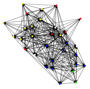
CETIS and JISC Innovation Group Twitter follower network. Colours indicate the team and arrows show the "follows" relationship in the direction of the arrow.
Nonplussed? What of the hypotheses?
Well… I suppose it is possible to assert that this is quite a dense network that seems to show a lot of mutuality and, assuming the Fruchterman-Reingold layout algorithm hasn’t distorted reality, which shows some hints at team cohesiveness and a few less-connected individuals. I think JISC management should be quite happy with the implications of this picture, although it should be noted that there are some people who do not use Twitter and that this says nothing about what Twitter mediates.
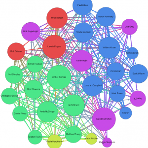
A little more attention to the visualisation can reveal a little more. The graph below (which is a link to a full-size image) was created using Gephi with nodes coloured according to team again but now sized according to the eigenvector centrality measure (area proportional to centrality), which gives an indication of the influence of that person’s communications within the given network.

Visualising the CETIS and JISC Innovation network with centrality measures. The author is among those who do not tweet.
This does, at least, indicate who is most, least and middling in centrality. Since I know most of these people, I can confirm there are no surprises.
Trying out several candidate models in order to try to decide on the previously enumerated hypotheses (and some others omitted for brevity) leads to the following tentative conclusions, i.e. to a model that appeared to be consistent with the observed network. “Appeared to be consistent” means that my inexperienced eye considered that there was acceptable goodness of fit between a range of statistics computed on the observed network and ensembles of networks simulated using the given model and best-fit parameters.
Keeping the same numbering as the hypotheses:
- ERGM isn’t needed to judge network density but the method does show the degree to which connections can adequately be put down to pure chance.
- There is indeed a large positive coefficient for mutuality, i.e. that reciprocal “follows” are not just a consequence of chance in a relatively dense network.
- It is not possible to make conclusions about organisational hierarchy.
- There is a statistically significant greater density within teams. i.e. team homophily seems to be affecting the network. This seems to be strongest for the Digital Infrastructure team, then CETIS then the eLearning team but the standard errors are too large to claim this with confidence. The two other teams were considered too small to draw a conclusion
- None of CETIS, the eLearning team or the Digital Infrastructure team seem to be more sociable. The two other teams were considered too small to draw a conclusion. This is known as a “main effect”.
- There is no statistically significant preference for certain teams to follow each other. In the particular case of CETIS, this makes sense to an insider since we have worked closely with JISC colleagues across several teams.
One factor that was not previously mentioned but which turned out to be critical to getting the model to fit was individual effects. Not everyone is the same. This is the same issue as was outlined for the EC-TEL 2012 followers: heterogeneity. In the present case, however, only a minority of people stand out sufficiently to require individual-level treatment and so it is reasonable to say that, while these are necessary for goodness of fit, they are adjustments. To be specific, there were four people who were less likely to follow and another four who were less likely to be followed. I will not reveal the names but suffice to say that, surprising though the results was at first, it is explainable for the people in CETIS.
A Technical Note
This is largely for anyone who might play with the R package. The Twitter rules prevent me from distributing the data but I am happy to assist anyone wishing to experiment (I can provide csv files of nodes and edges, a .RData file containing a network object suitable for use with the ERGM package or the Gephi file to match the picture above).
The final model I settled on was:
twitter.net ~ edges +
sender(base=c(-4,-21,-29,-31)) +
receiver(base=c(-14,-19,-23,-28)) +
nodematch("team", diff=TRUE, keep=c(1,3,4)) +
mutual
This means:
- edges = > the random chance that A follows B unconditionally on anything.
- sender => only these four vertices are given special treatment in terms of their propensity to follow.
- receiver => special treatment for propensity to be followed.
- nodematch => consider the team attribute for teams 1, 3 and 4 and use a different parameter for each team separately (i.e. differential homophily).
- mutual => the propensity for a person to reciprocate being followed.
And for completeness the estimated model parameters for my last run. The parameter for “edges” indicates the baseline random chance and, if the other model elements are ignored, an estimate of -1.64 indicates that there is about a 16% chance of a randomly chosen A->B tie being present (the estimate = logit(p)). The interpretation of the other parameters is non-trivial but in general terms, a randomly chosen network containing a higher value statistic for a given sub-graph type will be more probable than one containing a lower value when the estimated parameter is positive and less probable when it is negative. The parameters are estimated such that the observed network has the maximum likelihood according to the model chosen.
                         Estimate Std. Error MCMC %  p-value
edges                     -1.6436     0.1580      1  < 1e-04 ***
sender4                   -1.4609     0.4860      2 0.002721 **
sender21                  -0.7749     0.4010      0 0.053583 .
sender29                  -1.9641     0.5387      0 0.000281 ***
sender31                  -1.5191     0.4897      0 0.001982 **
receiver14                -2.9072     0.7394      9  < 1e-04 ***
receiver19                -1.3007     0.4506      0 0.003983 **
receiver23                -2.5929     0.5776      0  < 1e-04 ***
receiver28                -2.5625     0.6191      0  < 1e-04 ***
nodematch.team.CETIS       1.9119     0.3049      0  < 1e-04 ***
nodematch.team.DI          2.6977     0.9710      1 0.005577 **
nodematch.team.eLearning   1.1195     0.4271      1 0.008901 **
mutual                     3.7081     0.2966      2  < 1e-04 ***
---
Signif. codes:  0 ‘***’ 0.001 ‘**’ 0.01 ‘*’ 0.05 ‘.’ 0.1 ‘ ’ 1
Outlook
The point of this was a learning experience; so what did I learn?
- It does seem to work!
- Size is an issue. Depending on the model used, a 30 node network can take several tens of seconds to either determine the best fit parameters or to fail to converge.
- Checking goodness of fit is not simple; the parameters for a proposed model are only determined for the statistics that are in the model and so goodness of fit testing requires consideration of other parameters. This can come down to “doing it by eye” with various plots.
- Proper use should involve some experimental design to make sure that useful attributes are available and that the network is properly sampled if not determined a-priori.
- There are some pathologies in the algorithms with certain kinds of model. These are documented in the literature but still require care.
The outlook, as I see it, is promising but the approach is far from being ready for “real users” in a learning analytics context. In the near term I can, however, see this being applied by organisations whose business involves social learning and as a learning science tool. In short: this is a research tool that is worthy of wider application.
This is an extended description of a lightning talk given at the inaugural SoLAR Flare UK event held on November 19th 2012. It may contain errors and omissions.

