A good thing about working in JISC CETIS is being surrounded by the wide array of interests and ideas of its staff. A bad thing about working for JISC CETIS is with its distributed nature (and the fact everybody is always so busy!) it is always not possible to sit down and have a good natter about these interests.

Sheila recently blogged about social analytics and the way people share things. I enjoyed the post as I find resource sharing online a really interesting area. I increasingly find myself getting anxious about how I share things online and to which online persona ideas and resources are attached. I find myself carving out an online identity created of different levels of obscurity where I push my outputs up the levels as and when I feel more comfortable with them. I find it interesting that Christopher Poole’s latest social network allows you to work anonymously and then gives you the option to claim the work at a later date.

I left a comment on Sheila’s post and she replied back to me. First through a comment back on the post followed up by a quick skype chat. It occurred to me then that an online social structure that has worked very well for me has been the JISC CETIS blogs. An environment of regular blogging and commenting allows ideas to be shared and grow through the distributed organisation.

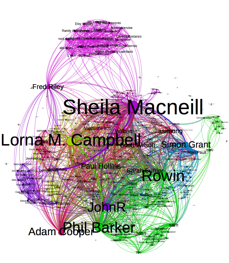
Over the past week or so I’ve been collecting data for a report and struggling with a way to analyse it. I came up with a method of turning networks I can spot in my CSV files into something network analysis tools can understand (which you can read about further down the chain of obscurity). Now that I’m obsessed with running data through the technique I thought I’d run CETIS blog authors and the conversations that join them over the method and steal Tony’s visualisation technique. I’ve removed pingbacks and such. It might not be useful but it tickles the occipital lobe.

I have been poking around Adam Coopers text mining weak signals in R code, and being too lazy to collect data in CSV format wondered if I could come up with something similar that used RSS feeds. I discovered it was really easy to read and start to mine RSS feeds in R, but there didn’t seem to be much help available on the web so I thought I’d share my findings.

My test case was the new CETIS publications site, Phil has blogged about how the underlying technology behind site is wordpress, which means it has an easy to find feed. I wrote a very small script to test things out that looks something like this:

      library("XML")
      library("tm")
      doc<-xmlTreeParse("http://publications.cetis.org.uk/feed") 
      src<-xpathApply(xmlRoot(doc), "//category")
      tags<- NULL

      for (i in 1:length(src)) {
             tags<- rbind(tags,data.frame(tag=tag<-xmlSApply(src[[i]], xmlValue)) )  
      }

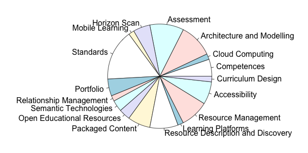
This simply grabs the feed and puts all the categories tags into a dataframe. I then removed the tags that referred to the type of publication and plotted it as a piechart. I’m pretty sure this isn’t the prettiest way to do this, but it was very quick and worked!

         cats <- subset(tags, tag != "Briefing Paper" & tag != "White Paper" & tag != "Other Publication" & tag != "Journal Paper"  & tag != "Report")
         levels(cats$tag)
         df$tag = factor(df$tag)
         pie(table(cats$tag))

Which gave me a visual breakdown of all the categories used on our publications site and how much they are used:

I was surprised at how much of a 5 minute job it was. It struck me that because the feed has the publication date it would be easy to do the Google Hans Rosling style chart with it. My next step would be to grab multiple feeds and use some of Adams techniques on the descriptions/content of the feed.

*UPDATE*

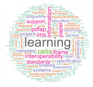
I had been interested in how to grab RSS and pump it into R and ‘interesting things we can do with the CETIS publications RSS feed’ had been a bit of an after thought. Martin brought up the idea of using the feed to drive a wordl (see comments). I stole the code from the comment and changed my code slightly so that I was grabbing the publication descriptions rather than the tags used… This is what it came up with.. Click to enlarge

I attended the SNA session at the CETIS conference hosted by Lorna, Sheila, Tony and Martin. Before the session I had blogged about some of the questions I had on SNA and although I think I have more new questions than answers I feel like things are much clearer now. My mind is still going over the conversations that were had at the session but these are the main themes and some early thoughts that I came away with.

What are the quick wins?
At the start of the session Sheila asked the question ‘What are the quick wins?’.   While Tony and Martins presentations were excellent I think it is hard for people who don’t have their head regularly in this space to replicate the techniques quickly. Lorna said that although she understood what was happening in the SNA examples there was some ‘secret magic that she couldn’t replicate when doing it for herself, Tony agreed that when you work in this area for a while you start to develop a workflow and understand some of the quirks of the software. I could relate to Lorna’s dilema as it took me a few hours of using Gephi just to know exactly when I needed to force quit the program and start all over again.

So for people who want to find out useful information about social networks but don’t have the time to get into the secret magic of SNA can we develop quick and simple tools that answer quick and simple questions?

The crossover between data driven visualisations and SNA
The session helped me make a clear distinction between Data Driven Journalism and SNA . While there is a crossover between the two the reasons for doing them are quite different. SNA is a way to study social networks and data driven visualisations are a way to convey a story to an audience. Although the two do cross over I found that making distinctions between them both helped me get to grips with the ‘why is it worth doing this’ question.

Data Validation
Martin made the point that when he was playing with PROD data to create visualisations he found that it was a great way of validating the data itself as he managed to spot errors and feed that back to Wilbert and myself.

Lies, Damned Lies and Pretty Pictures
Amber Thomas did a fantastic presentation, if you missed the session it is available here. I felt Amber had really thought about the ‘How is this useful?’ question and I felt lots of pieces of the puzzle click into place during the presentation. I really recommend spending the time to go through the slides.

Thanks to Sheila, Lorna, Amber, Tony and Martin for an interesting session.

Today I took part in an introduction to R workshop being held at The University of Manchester. R is a software environment for statistics  and while it does all sorts of interesting things that are beyond my ability one thing that I can grasp and enjoy is exploring all the packages that are available for R, these packages extend Rs capabilities and let you do all sorts of cool things in a couple of lines of code.

The target I set out for myself was to use JISC CETIS Project Directory data and find a way of visualising standards used in JISC funded projects and programmes over time. I found a Google Visualisation package and using this I was surprised at how easy it was to generate an output , the hardest bits being manipulating the data (and thinking about how to structure it).  Although my output from the day is incomplete I thought I’d write up my experience while it is fresh in my mind.

First I needed a dataset of projects, start dates, standards and programme. I got the results in CSV format by using the sparqlproxy web service that I use in this tutorial and stole and edited a query from Martin

Sparql:

PREFIX rdfs:
PREFIX jisc:
PREFIX doap:
PREFIX prod:
SELECT DISTINCT ?projectID ?Project ?Programme ?Strand ?Standards ?Comments ?StartDate ?EndDate
WHERE {
?projectID a doap:Project .
?projectID prod:programme ?Programme .
?projectID jisc:start-date ?StartDate .
?projectID jisc:end-date ?EndDate .
OPTIONAL { ?projectID prod:strand ?Strand } .
# FILTER regex(?strand, “^open education”, “i”) .
?projectID jisc:short-name ?Project .
?techRelation doap:Project ?projectID .
?techRelation prod:technology ?TechnologyID .
FILTER regex(str(?TechnologyID), “^http://prod.cetis.org.uk/standard/”) .
?TechnologyID rdfs:label ?Standards .
OPTIONAL { ?techRelation prod:comment ?Comments } .
}

From this I created a pivot table of all standards, and how much they appeared in each projects and programmes for each year (using the project start date). After importing this into R, it took two lines to grab the google visualisation package and plot this as Google Visualisation Chart.

library(“googleVis”)
M = gvisMotionChart(data=prod_csv, idvar=”Standards”, timevar=”Year”, chartid=”Standards”)

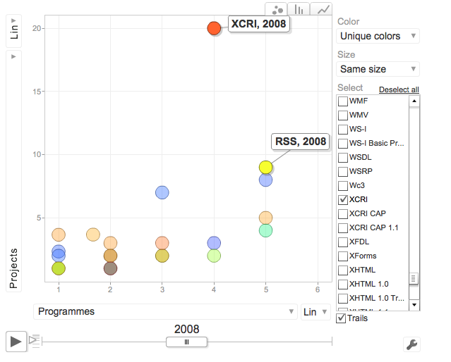
Which gives you the ‘Hans Rosling’ style flow chart. I can’t get this to embed in my wordpress blog, but you can click the diagram to view the interaction version. The higher up a standard is the more projects it is in and the further across it goes the more programmes it spans.

Some things it made me think about:

1. Data from PROD is inconsistent

Standards can be spelt differently; some programmes/projects might have had a more time spent on inputting related standards than others

2. How useful is it?

This was extremely easy to do, but is it worth doing? I feel it has value for me because its made me think about the way JISC CETIS staff use PROD and the sort of data we input. Would this be of value to anybody else?  Although it was interesting to see the high number of projects across three programmes that involved XCRI in 2008.

3. Do we need all that data?

There are a lot of standards represented in the visualisation. Do we need them all? Can we concentrate on subsets of this data.